In this chapter, we’ll look at what is called thehistogram of an image.
We will discover also two algorithms to automatically improve the quality of an image by controlling the distribution of its pixels.
Histogram of an image
Statistics in image processing
As I told you in the chapter what is an image we can set an image as a function of which we do not know the formula, but in which we can observe the result on a given set of values (in this case, a plane). There is a branch of mathematics that focuses on the study of this kind of functions as ” black boxes “, and you’ve probably already addressed (but not necessarily from this angle there) : statistics.
In fact, when the statistics from a formal point of view (in general, this goes hand in hand with the probabilities), we model the phenomena that one is studying functions of which we can only observe the result, giving them the name of random variables. The aim of the game is to extract information from these variables by observing data that describe their behaviour.
Rest assured though, this does not mean that we’re going to do probability or statistics in this chapter ; this note on the analogy between the images and the random variables is mainly there to explain to you that it is possible (and relatively common) to use concepts and tools from statistics to image processing. The histogram is one of these tools.
Histogram and cumulated histogram
Histogram
In statistics, a histogram is a graph that is used to observe the distribution of values that takes a random variable. In our case, we will use it to observe the distribution of values taken by the pixels of an image.
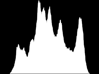
Specifically on an image single-channel 8-bit, this means that we will count, for each level of gray $i$ between 0 and 255, the number of pixels that carry the value $i$. It should be noted this number $h_i$. We can then represent this histogram by a bar chart, which takes on the abscissa values $i$ (from 0 to 255, so), and on the ordinate the $h_i$corresponding.
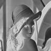
For example, for the image of Lena inverted grayscale :
We get the histogram below :
As for the following image, which is very dark (what we’ll address in the rest of this chapter…) :
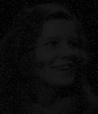
We obtain a histogram “shrunken” to the left, that is to say, to the gray levels closest to the black :
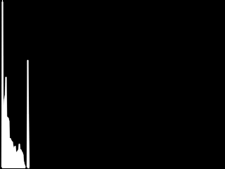
This diagram is, therefore, clearly show how the distribution of the gray levels in the image.
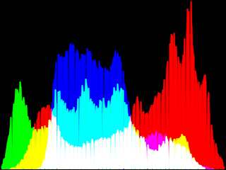
Of course, we can also draw a histogram of a color image, by overlaying the histograms of its channels. For example, for Lena :
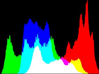
Cumulated histogram
In addition to the histogram classic, it can be interesting in some cases to work on the histogram accumulated. The latter is obtained by associating to each gray level $i$ the number $h_i^c$ of pixels of the image that have a value less than or equal to $i$. Somehow, we compute the histogram of the image and associate to each level $i$ the sum of $h_j$ for $j \leq i$.
In formula, this gives :
$h_i^c = \sum_{0 \leq j \leq i}{h_j} = h_0 + h_1 + \cdots + h_i$
On the image of lena reverse, this gives a curve that look like this :
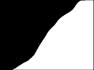
And the image is very dark :
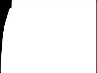
As you can see, the curve rises very quickly to 100%, whereas on a picture more ” watchable “, its slope is more steadily increasing.
Finally, here are the cumulated histogram of Lena-color :
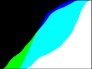
The advantage of the cumulated histogram is that it allows you to calculate very easily the number of pixels having a value between two gray levels given $a$ and $b$ simply to calculate the difference $h_b^c – h_a^c$ .
In mathematics, this is equivalent to calculating the integral of the histogram between the points $a$ and $b$ ; this is the reason for which the cumulated histogram is also called ” histogram integral “.
Calculation of a histogram
In order to return to the notions of histogram and cumulated histogram, let’s create a small function that calculate the histogram of a grayscale image, 8 bits.
/**
 * Calcule l'histogramme d'une image en niveaux de gris 8 bits
 * arguments:
 * - img: image dont on calcule l'histogramme
 * - bins: tableau destiné à contenir l'histogramme
 * - cumul: 1 pour l'histogramme cumulé, 0 sinon
 * retourne:
 * la valeur maximale de l'histogramme
 */
long compute_hist_8U (const IplImage* img, long* bins, int cumul);
This function expects as second argument an array that is already allocated, for instance in the following way :
long bins[256];
Here is the code :
#include <strings.h>
#include <opencv/cv.h>

long compute_hist_8U (const IplImage* img, long* bins, int cumul)
{
  uchar *p, *line;
  long* b;
  long max = 0;

  assert (img->nChannels == 1);
  assert (img->depth == IPL_DEPTH_8U);

  /* initialisation du tableau "bins" */
  memset (bins, 0, 256 * sizeof(long));

  /* calcul de l'histogramme et de sa valeur maximale */
  for (line = (uchar*) img->imageData;
       line < (uchar*) img->imageData + img->imageSize;
       line += img->widthStep)
  {
    for (p = line; p < line + img->width; ++p)
    {
      /* Pour chaque pixel, on incrémente le compteur
       * correspondant à son niveau de gris.
       * On met à jour la variable "max" si besoin.
       */
      if (++bins[*p] > max)
      {
        max = bins[*p];
      }
    }
  }

  /* calcul de l'histogramme cumulé */
  if (cumul)
  {
    for (b = bins; b < bins + 255; ++b)
    {
      *(b+1) += *b;
    }
  }
  /* la valeur max d'un histogramme cumulé est nécessairement
   * la dernière.
   */
  return (cumul ? bins[255] : max);
}
We will use this function when we are going to implement the equalization of histograms.
Normalization of an image
It happens that some of the real images are too dark or too bright, a little like the following in an extreme case :

As I showed you a little over the top, the histogram of this image is found all flattened in the area of values dark :

This is explained by the fact that in this image, the gray levels do not occupy the entire interval of values that they can take. Instead, they are all included between two values $\mathrm{min}$ and $\mathrm{max}$ such that $0 \leq \mathrm{min} < \mathrm{max} < 256$.
To remedy this, we can simply try to normalize this image, that is to say, to adjust the scale of levels of gray so that it occupies the whole available range. To put it simply, it is a question of applying a rule of three to the pixels of the image, which are all included in the interval $\left[\mathrm{min}, \mathrm{max}\right]$, to adjust the interval $\left[0,255\right]$.
This rule of proportionality is given by the following formula :
$\mathrm{dst}(x,y) = \dfrac{\left(\mathrm{src}(x,y) – \mathrm{min}\right) \times 255}{\left(\mathrm{max} – \mathrm{min}\right)}$
If we apply mentally the operations in the order, we realize that this treatment begins by bringing back all values from interval $\left[\mathrm{min}, \mathrm{max}\right]$ to interval $\left[0, \mathrm{max}-\mathrm{min}\right]$, and then it extends these values to $\left[0,255\right]$.
Manual implementation
Try to implement this treatment ourselves, for a grayscale image. It seems clear that the algorithm consists of two steps :
-
First, it determines the values $\mathrm{min}$ and $\mathrm{max}$ the gray levels of the image ;
-
Then, we apply the formula that we have seen.
Although OpenCV may already have these two functions, here’s how we could do this “manually” :
void normalize_manual (IplImage* img)
{
  double scale;
  uchar min = 255, max = 0;
  uchar *p, *line;

  assert (img->depth == IPL_DEPTH_8U);
  assert (img->nChannels == 1);

  /**
   * Recherche des valeurs min et max,
   * et calcul du facteur d'échelle
   */
  for (line = (uchar*) img->imageData;
       line < (uchar*) img->imageData + img->imageSize;
       line += img->widthStep)
  {
    for (p = line; p < line + img->width; ++p)
    {
      if (*p < min) min = *p;
      if (*p > max) max = *p;
    }
  }

  scale = 255.0 / (max - min);

  /**
   * Normalisation des niveaux de gris
   */
  for (p = (uchar*) img->imageData;
       p < (uchar*) img->imageData + img->imageSize;
       ++p)
  {
    *p -= min;
    *p *= scale;
  }
}
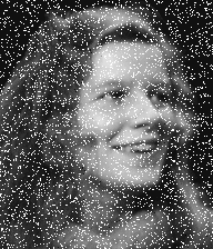
Here is the result you should get :
And here is its histogram :
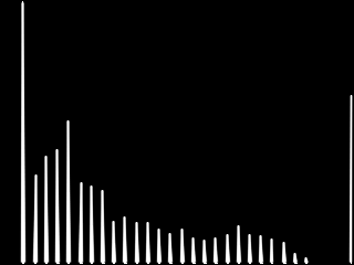
I guess you now understand why the normalization of an image is also called ” histogram stretching “.
Use OpenCV
Although the previous function is in itself quite simple, it is good to have the reflex to ask systematically whether the basic operations that we perform are not already implemented by OpenCV. Here, the answer is obviously ” yes “.
To find the minimum and maximum values of gray levels of an image, OpenCV offers us the function cvMinMaxLoc :
/**
 * Recherche des niveaux de gris min et max d'une image.
 * Arguments:
 * - arr : l'image
 * - minVal : pointeur sur la valeur min
 * - maxVal : pointeur sur la valeur max
 * - minLoc : pointeur sur le premier point de l'image de valeur min
 * - maxLoc : pointeur sur le premier point de l'image de valeur max
 * - mask :   masque optionnel déterminant la zone de l'image,
 *            où effectuer la recherche
 */
void cvMinMaxLoc (const CvArr* arr, double* minVal, double* maxVal,
                  CvPoint* minLoc, CvPoint* maxLoc, const CvArr* mask);
The last three arguments to this function are optional. In our case, we will be able to leave NULL.
Thus, we can replace the first loop of our function by this :
double min, max;
cvMinMaxLoc (img, &min, &max, NULL, NULL, NULL);
For the application of a scale factor, we have at our disposal the following function :
/**
 * Changement d'échelle d'une image selon la formule :
 * dst(x,y) = alpha * src(x,y) + beta
 *
 * arguments :
 * - src : image source
 * - dst : image destination
 * - alpha, beta : paramètres de la formule
 */
void cvScale (CvArr* src, CvArr* dst, double alpha, double beta);
To use this function in our case, we’re going to need to modify our formula to determine the settings alpha and beta, like this :
$\begin{align}\mathrm{dst}(x,y) &= \dfrac{\left(\mathrm{src}(x,y) – \mathrm{min}\right) \times 255}{\left(\mathrm{max} – \mathrm{min}\right)} \\&= \mathrm{src}(x,y) \times \underbrace{\left(\dfrac{255}{\mathrm{max} – \mathrm{min}}\right)}_{\alpha} – \mathrm{min} \times \left(\dfrac{255}{\mathrm{max} – \mathrm{min}}\right)\\&= \mathrm{src}(x,y) \times \alpha + \underbrace{\left(- \mathrm{min}\right) \times \alpha}_{\beta}\\&= \alpha \times \mathrm{src}(x,y) + \beta\;,\end{align}$
where the values :
$\begin{align}\alpha &= \dfrac{255}{\mathrm{max} – \mathrm{min}}\;,\\\beta &= \left(- \mathrm{min}\right) \times \alpha\;.\end{align}$
This brings us to the complete function follows :
void normalize_gray (IplImage* img)
{
  double min, max, alpha, beta;

  assert (img->depth == IPL_DEPTH_8U);
  assert (img->nChannels == 1);

  cvMinMaxLoc (img, &min, &max, NULL, NULL, NULL);

  alpha = 255.0 / (max - min);
  beta  = -min * alpha;
  cvScale (img, img, alpha, beta);
}
As you might expect, we can generalize this treatment to color images by applying the method split & merge. I leave it to you to implement this treatment as exercise.
Here are the results on lena (before/after) :
As well as the histograms associated :

Histogram equalization
It may happen that the pixels in an image, while occupying the whole space of values available between 0 and 255, are ” stuck “, that is to say that the histogram is not uniform. This is the case, for example, photographs that are backlit like the following :
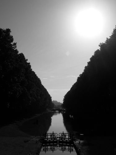
What jumps very quickly to the eyes, it is that this image contains many pixels of very dark or very clear, and relatively few pixels of a brightness ” in average “. Here is the histogram and cumulated histogram of this photograph :
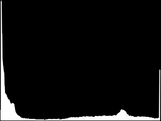
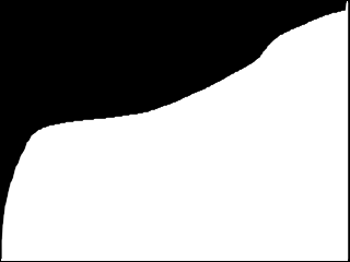
As you can see, all the space of values available is already used, the standards would, therefore, have strictly no effect on this image. It is here that comes into play with the histogram equalization, the goal of which is to standardize the distribution of pixel values, that is to say, to obtain an image that contains roughly the same amount of pixels and very dark pixels means that pixels are very clear, and of which the cumulated histogram would look something like this :
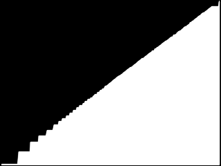
To do this, we’re going to retro-project the cumulated histogram of the original image. This term may seem barbaric, but you will see that it in reality hides a trick quite magical, which is summarized by the following formula :
$\mathrm{dst}(x,y) = h_{\mathrm{src}(x,y)}^c$
Equalizer algorithm
To equalize the histogram of an image, we start by calculating the cumulated histogram of this image, and we standardize its values between 0 and 255.
Then comes the phase of retro-projection. For each pixel of the image, it retrieves the value of the cumulated histogram associated with level of grey that he wears. In normal times, the cumulated histogram should contain the number (or percentage) of pixels of the image that are darker than him. Here, we give a ranking, between 0 and 255, where it will replace the pixel.
For example, if 60% pixels of the image are darker than the gray level 40 (which means that the image contains many dark pixels), it will replace all the pixels with the level 40 $h_{40}^c = 0.6 \times 255 = 153$. This will have the effect of enhancing the contrast in the dark areas of the image.
Here is an implementation of this algorithm :
void equalize_gray (IplImage* img)
{
  long bins[256];
  double ratio;
  uchar* p;

  assert (img->nChannels == 1);
  assert (img->depth == IPL_DEPTH_8U);

  ratio = 255.0 / (img->height * img->width);

  /* calcul de l'histogramme cumulé */
  compute_hist_8U (img, bins, 1);

  /* rétro-projection de l'histogramme sur l'image */
  for (p = (uchar*) img->imageData;
       p < (uchar*) img->imageData + img->imageSize;
       ++p)
  {
    *p = bins[*p] * ratio;
  }
}
And now here is the result on the previous photo :
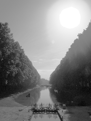
As you can see, the histogram equalization shows a lot of details that were invisible to the naked eye in the darkest areas of the image, such as piece of forest to the left and its reflection in the water. These details were already included on the original image, but the very high brightness of the rest of the scene has pushed the mechanism of white balance of the camera to assign to those pixels values much lower than normal.
To the right of the image, on the other hand, the much less details have emerged, giving way to the noise. Typically, this is due to the sun’s rays that hit the sensor more directly to this place, “dazzling” and the light-sensitive cells.
No miracle, therefore. This algorithm, while simple, does not reveal the details already captured by the device at the time of the shooting, and naturally cannot replace a sensor of good quality.
As for standardization, I’ll leave as an exercise the task of implementing a function of the equalization on color images. You can use the following function from OpenCV :
/**
 * Égalisation de l'histogramme d'une image en niveaux de gris.
 */
cvEqualizeHist(CvArr* src, CvArr* dst);
You can as well amuse you to equalize all the images that you spend on hand, and make it appear so horribly visible defects of jpeg compression.
We have just discovered two treatments that are intended to reveal details on the most natural images. As you may realize on the examples that I have used in this chapter, there is unfortunately not as interesting details become visible, but also a lot of noise.
This is the reason why we’re going to discover, in the next chapters of this part, several methods of “filtering” to eliminate at best the noise of the images.
This tutorial is being written.

